Determination of Flood Extent Using Remote Sensing

Introduction

Flood is a relatively high flow of water that overtops the natural and artificial banks in any of the reaches of a stream. When banks are overtopped, water spreads over flood plain and generally causes problem for inhabitants, crops and vegetation. During extreme flood event it is important to determine quickly the extent of flooding and landuse under water (Wang et al, 2002). Flood map can be applied to develop comprehensive relief effort immediately after flooding. There are varieties of issues and uncertainties involved in flood mapping. Remotely senses data can be used to develop flood map in an efficient and effective way. In this paper the different techniques of flood mapping using active and passive remote sensing system applied by different researchers will be presented with their specific application. Finally a comparison of different methods will be made.

Figure 1: 2007 Global Flooding (Dartmouth Flood observatory)

• Data Requirement for Flood Mapping

Generally for flood mapping two sets of remotely sensed data are required; one set consisting of data acquired before the flood event and the other acquired during the flood occurrence (Wang et al., 2002). The image before the flood usually used as the reference. Sometimes two reference images acquired for finding out the mean reference DN values of pre flood scenarios. However aerial photographs, DEM, water level measurements and high water marks after flood events are required for the aid of analysis. The remote sensing data may be provided by the active or passive remote sensing system. In some of the studies a combination of active and passive remotely sensed data is used (Imhoff et al., 1987).

• Difficulties

1. Flood is a wave phenomenon and all satellites have their repeating intervals. So generally the time of acquisition of satellite data does not coincide with the time of flood peak which is related to the maximum inundation area (Islam and Sado, 2000a).
2. In most of the cases timely acquisition of flood data is prevented by the obscuring cloud cover, especially in the monsoon countries where flooding occurs due to widespread precipitation over relatively long period of time (Imhoff et al., 1987). Usually passive remote sensing system as NOAA AVHRR, LandSat MSS, LandSat TM cannot receives the radiance from a cloud covered ground surface. So presence of cloud cover over the flooded area limits the usefulness of these data and difficulties arises with the interpretation of whether a given area beneath cloud cover is dry or water (Imhoff et al., 1987, Islam, M.M. and Sado, K., 2002, Wang et al., 2002).
3. Due to the lack of canopy penetration of Landsat TM data, flooded areas under dense canopies may not be detected by the classification of the TM data which results the underestimation of the flooded area ( Wang et al., 2002).
4. Active remote sensing system as SAR has the capability of allowing delineation of flood boundary beneath cloud cover, vegetation canopies but actual application of SAR however frustrated due to a lack of regularly available data such as might be achieved using space borne SAR platforms. Aerial acquisition of SAR data also limited by the bad weather condition and the aerial extent (Imhoff et al., 1987).

• Objectives

1. To review the methodologies of delineation of flood boundary using passive and active remote sensing system
2. To compare the different methods with respect to their specific capabilities and limitations in application.

Flood Mapping by Passive Remote Sensing System

• General

Passive remote sensing data have been widely used for flood mapping. Imhoff et al. (1987) used Landsat MSS data to delineate flood boundaries by monsoon rains in Bangladesh, Islam and Sado (2000a, 2002) used NOAA AVHRR data for mapping the extent of flood and food hazard map of Bangladesh, Wang et al. (2002, 2004) used Landsat TM to delineate the maximum flood extent on a coastal flood plain of North Carolina, USA. The methodology applied by Wang et al (2002) will be presented below as an example of flood delineation using passive remote sensing data. The reasons of choosing this method are a) TM data are more appropriate than AVHRR data for flood mapping because of coarser resolution of AVHRR b) the method is efficient and economic c) it combines the DEM with TM data to delineate flood boundary in forested region as TM data has the limitation in distinguishing flooded area in forest canopies.

• Methodology

• Identifying water verses non water areas

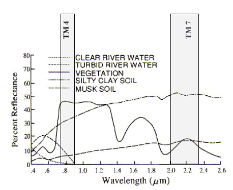
Figure 2: Spectral reflectance of vegetation, soil and water (Remote Sensing Notes, 1999)

The first task of food mapping is identifying the water verses non water areas for the reference image and the flooded image. Two steps should be followed are:

i) Representation of the reflectance values of water and non water feature

Here it should be noted that water has almost no reflectance in the infrared region. Referring to the Figure 2 it is obvious that TM 4 (0.76-0.90 μm) is responsive to the amount of vegetation biomass where is water has almost no reflectance in this band. So TM 4 band is useful in identifying land and water boundaries. But confusion arises between the reflectance of water with asphalt areas i.e. road pavement and rooftops of building as they reflect little back to sensor and appeared black on the TM 4 image. It was found that on the TM 5 and TM 7 (2.08-2.35 μm) image the reflectance of water, paved roof surfaces and rooftops are different. But the differences are slightly smaller in TM 5 than those are in TM 7. So the addition of TM 4 and TM 7 (TM 4+TM 7) will be useful for determining water verses non water area. So if the reflectance of a pixel is low in TM 4+TM 7 image the pixel is considered as water, otherwise it will represented as non water

ii) Setup the cutoff value

After the representation of the reflectance of the water and non water features, a cutoff value of DN has to be set to separate the water and non water features. Say this cutoff value is DNc. So if a pixel’s DN value is less than DNc, the pixel will be categorized as water otherwise it would be assigned as non water. The selection of cutoff values might be done by ground truthing and by histogram analysis of the (TM 4 + TM7) image. Ground truthing involves taking observation directly form the field and through the analysis of aerial photos.

• Determining flooded area during the flood event

After identifying water and non water area on the before flood and during flood image the flood affected area could be made. Both of the images should be examined in a pixel to pixel basis.

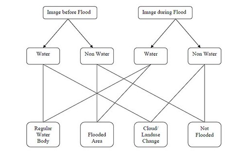
Figure 3: Determination of flooded and non flooded area

There are four possible scenarios as shown in Figure 3:

• Water-Water: If a pixel is classified as water on the pre-flood image and water on the during flood image the pixel is not be considered as flooded, rather the pixel represents the regular water body as streams, lakes etc.
• Non Water-Water: If a pixel is classified as non water on the pre-flood image and water on the during flood image the pixel will be considered as Flooded.
• Non Water-Non Water: If a pixel is classified as non water on the both image, the pixel will be considered as Non flooded
• Non Water-Water: If a pixel is found that is classified as non water on the pre flood image but water on during flood image the pixel might be considered as changes in landuse during period of image acquiring or cloud.

• Application Study

The methodology of flood delineation as discussed above was applied by Wang et al. (2002) for mapping flood extent in a coastal flood plain of North Carolina, USA. The summary of the study will be discussed in the following sections.

• Study area and flood occurrence

The study area is the city of Greenville, Pit County which situated on the south side of the Tar River. Pit County lies in the eastern coastal plain of North Carolina. There are four large rivers system that drain the coastal plain in a north-west-south-east direction. In 15 September 1999, Hurricane Floyd made landfall near South Carolina –North Carolina border and proceed to churn through eastern North Carolina. It causes 25-46 cm of rain in many areas within 72 hours results the Tar, Neuse, Roanoke and Pamlico rivers to reach their flood stage on 17 September. On 21 September Tar River reached its peak flood stage in the study area. Figure 4 shows an aerial photograph of the study area taken during the flood.

• Data collection

The Tar River peak discharge was reached on 21 September, 1999 which is related to maximum extent of the flood event. Due to the 16 days repeating period of Landsat 7 the pre-flood images were available on 14 September, 29 August, 13 August and 28 July. Among these the first three images had severe cloud coverage. The July image had some clouds and thin cloud patches but it was not so severe. So the July 28 image was selected as pre-flood image. The closest image after peak discharge was available on 30 September. So it was selected as during flood image. An aerial photograph during the flood was also collected and stage surface height of the water in the Tar River during the periods of mage acquiring was collected. High water marks data were collected for aid in ground truthing.

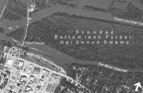
Figure 4: The study area during flood, September, 1999 (Wang et al, 2002)

• Flood Mapping

As mentioned in the methodology section, the reflectance of (TM 4+TM 7) image was examined for the 28 July and 30 September image. After ground thruthing and histrigram analysis a cutoff value of 141 was selected for the July image and 109 was selected for the September image. So any pixel having DN value less than 141 will be represented as water on the July image where as any pixel having DN value less than 109 will be considered as water in September image. So based on these cutoff values both images were classified as water and non water. After identifying water and non water areas both images were examined on a pixel by pixel basis. So the pixels classified as water on the both image was considered as regular river and ponds, whereas the pixels classified as non water on the both images was considered as non flooded areas. The flooded areas are classified as those pixels that were considered as non water on the July image and water on the September image. There were some pixels that were classified as water on the July images but non water on September image was considered as clouds.

• Results

Figure 5 represents the resulting flood extent map derived form the methodology as discussed in the previous sections. The flooded areas are shown in red and regular channels and pond are in blue. There are some yellow regions classified as clouds and the grey areas represent non flooded regions.

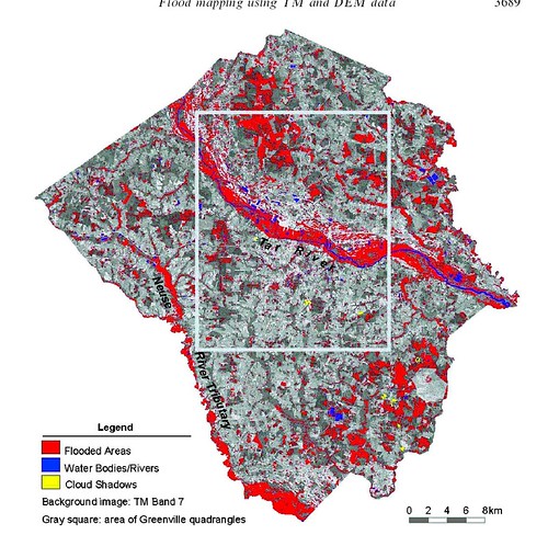
Figure 5: Flood extent in Pit County, NC on 30 September, 1999 (Wang et al., 2002)

• Effect of Data acquisition date on Flood Mapping

As discussed earlier due to a fixed satellite orbit, it is almost impossible to have remotely sensed data concurrent with a flood peak event. This lake of timelines may undervalue the possible usage of satellite data for flood mapping (Wang, 2004). In the study of Wang (2002) the image during flooding was acquired 9 days after the peak flood discharge. It was observed that the Tar River water surface decreased from 8.32 m (above mean sea level) on 21 September 1999 to 5.34 m on 30 September 1999 (Wang, 2004). So a study was taken to investigate this effect. The details of the study will be available in Wang (2004); here the summary will be presented. Dataset used in the previous study (Wang et al., 2002) was acquired from Landsat 7 path 15/row 35. It was found that on 23 September 1999 i.e. 2 days after flood peak a image is available for path 14/row35 which has an overlap on the study area. So the flood mapping of the overlapping area was performed using July 28 data as reference and September 23 and September 30 data as two flood image. The methodology of flood mapping was almost same as the previous study except they use the TM 4+ TM 8 band to classify the pixels as water and non water. To facilitate the accuracy analysis 40 flooded sites and 45 non flooded sites were chosen for ground thruthing. Figure 6 shows the results. Comparing the flood map of 23 September and 30 September pixel by pixel, it was found that two maps are spatially in agreement of 90.7% . 6.7 % of the area involves the pixels that are classified as flooded on 23 September but as non flooded on 30 September. This 6.7% area may indicate the underestimation of flooded area. Remaining 2.6 % of the study area ware classified as non flooded on 23 September image and as flooded on 30 September image. The authors conclude these scattered pixels as local pooling. In an acuracy analysis they showed that the overall accuracy of the flood map is between 82.5% and 89.7% , whereas the accuracy of determining flooded and non flooded open areas is 96%. The decrease in overall accuracy is due to the presence of some forest areas in the study area in agreement with the inability of TM sensor to penetrate through dense forest canopies.

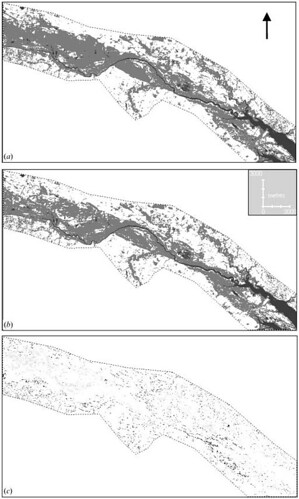
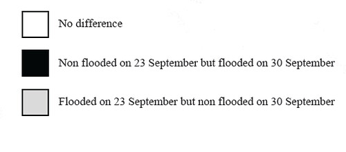
Figure 6: Inundation maps of 23 September 1999 (a), 30 September 1999 (b) and comparison of two maps (c) (Wang, 2004)

Flood Mapping by Active Remote Sensing System

• General

Active remote sensing system as Synthetic Aperture Radar (SAR) system is very useful for mapping floods because of their all weather functionality, their independency from sun as the illumination source and ability of penetrate through forest canopy at a certain frequencies and polarization (Lawrence et al., 2005, Townsend, 2002). Airborne and space borne SAR system offers high resolution views of flood inundation extent devoid of cloud cover compared to TM or MSS. Imhoff et al.(1987) showed that SAR imagery can be more effective than Landsat MSS image for monsoon flood mapping in Bangladesh. Townsend (2002) derived the relationship between forest structure and flood inundation for lower Roanoke River floodplain in eastern North Carolina. Henry et al. (2006) used multi-polarized Advanced SAR data for flood mapping of Elbe river basin, Central Europe. Horrit et al. (2001) applied a statistical active contour model to delineate a flood from the SAR imagery. In this paper the methodology of applied by Lawrence et al. (2005) will be presented in the following sections together with the study of Henry et al. (2006).

• Methodology

In SAR system microwave radiation is produced which transmitted to the target object or area. The amount of microwave energy returned to the sensor is heavily dependent on the surface roughness and the dielectric constant of the elements. According to radar thumb rule, radar backscatter increases with the increases in the surface roughness and dielectric constant of the target. The wet and rough ground surface yield strong backscatter than the dry surface. As open water usually exhibit strong specular reflection away from the sensor, so they produce low backscatter and appear dark. The herbaceous vegetation also shows low backscatter on SAR image. The non herbaceous vegetation as forested swamps produces double backscatter during flooding and yield high backscatter. Considering those backscattering properties of water and harbeceous vegetation Lawrence et al. (2005) applied the following methodologies for delineate the flood boundary.

• Multi temporal image enhancement

This method is basically a system of producing color imagery based upon the additive characteristics of primary color. It involved taking of multi temporal black and white radar images adding them into RGB channels. The hue of the color indicates the date of change and the intensity of the color represents the degree of change. Usually two reference image i.e. pre flood image and one during flood image are used in analysis.

• Differencing of flood image from reference image

In this process the DN values of each pixel on the reference image or mean DN values of two or more reference images are subtracted from the DN values of the during flood image. The pixels having higher difference values indicated as flooded area and exhibit bright grey shades and dark pixels related to little or no change are considered as non flooded area.

• Application study

The methodology discussed in the previous sections was applied by Lawrence et al. (2005) for the mapping the hurricane related flooding of coastal Louisiana, USA. The summary of the study will be presented in the following sections.

• Study area and flood occurrence

The study area is a part of the vast wetlands of southern Louisiana which lies in the deltaic plain of Mississippi River. Within seven days in September/October 2002 the area was hit by two storm system, Tropical Storm Isidore and Hurricane Lili. Due to these storms extensive flooding were experienced along Louisiana coast. The peak flooding was occurred on 3 October 2002 as the coastal water level rose 100-300 cm over the Atchafalaya Bay. The study area is shown in Figure 7.

Figure 7: Map of Louisiana showing the study area and track of Hurricane Lili in October 2002(Lawrence et al., 2005)

• Data collection

A Radarsat SAR image was acquired on 3 October 2002, 8-9 hours after the peak water level. Two reference SAR images were collected on 23 and 28 September 2002. Also the water level data from 20 September to 8 October 2002 at different places over Atchafalaya delta region were collected.

• Flood mapping

Multi temporal image enhancement technique was applied to the data set acquired. Blue, green and red colors were assigned to 23 September, 28 September and 3 October SAR image. Another flood map was developed by applying the differentiating technique as discussed in the previous section. At first the Avegrage DN values of two reference image on 23 September and 28 September are calculated. Then these pixel DN values are subtracted from the during flood image on 3 October.

• Results

The color composite image is shown is Figure 8. The flooded areas are displayed as color cyan. The resulted absolute difference image is shown in Figure 9. The bright pixels are corresponding to flooding. In order to confirm the phenomena that brighter pixels in the difference image represents the flooded area six different sites are taken to carry out detail investigation. These sites appeared brighter on the difference image. The average backscatter (DN) values of these sites were obtained by randomly moving 9 X 9 pixel box over five different spots on each sites and computing mean backscatter values. Figure 10 shows the results. It was found that four sites show lower DN values on 3 October than on 23 and 28 September image. As lower backscatter corresponds to water body so the sites confirms the presents of flood water. Two sites show minimal changes in backscatter values in the 23 September, 28 September and 3 October image. It was concluded that those sites was experienced minimum inundation.

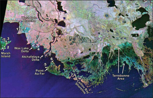
Figure 8: Multi-temporal color composite image with flooded sites. The color ‘cyan’ indicates marsh flooding on 3 October 2002. (Lawrence et al. 2005)

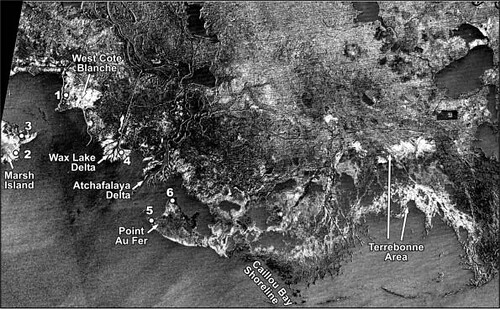
Figure 9: Difference image obtained by subtracting the mean DN values of 23 and 28 September 2002 SAR image from 3 October 2002 SAR Image (Lawrence et al. 2005)

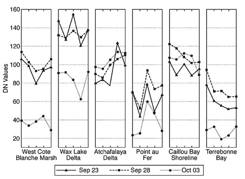
Figure 10: Summary of average backscatter (DN) values for six selected marsh sites in coastal Louisiana (Lawrence et al. 2005)

The relationship of the depth of flooding with SAR backscatter values was also studied. It was found that there is a direct correlation between the water level difference and the difference of DN values between the 3 October image (during flood image) and 23 September image (pre flood image). The relationship are shown in Figure 11.

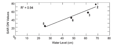
Figure11: Linear relationships between water levels (cm) SAR backscatter (DN) median values. The relationship based on SAR DN and water level differences from the flooding image and pre flooding image (Lawrence et al. 2005).

Application of multi polarized ASAR data for flood mapping

Multi polarized SAR data have been used for flooding mapping. Nghiem et al. (2000) used HH and VV polarized data for presenting a flood extent methodology. He used σHH/ σV V ratio and incident angle difference between pre flood and during flood image. Henry et al. (2006) used Envisat multi-polarized ASAR data for flood mapping of Elbe River basin. This method will be presented below:

Heavy rainfall over Central European alpine basin causes devastating flood on the Elbe River in August 2002 The peak flood flows over Elbe basin was occurred on 17 August 2002. In order to map the extent of flooding AP ASAR date were acquired on 19 August with HV and HH polarization combinations quasi-simultaneously with ERS-2 VV polarized data. It should be noted that both Envisat and ERS has the same resolution and incidence angle.

At first the statistics of three polarized data were analyzed. Figure 12 shows the histogram on overlapping areas of the three images. All these three histograms shows two peaks especially a small one found in the lower DN values of HH and VV datasets. So identifying flood inundation will be easier in like-polarized data than cross-polarized data. The wider histogram of HH data implies better possibility of HH data to identify thematic classes.

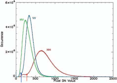
Figure 12: Value of occurrence for HH, HV and VV original dataset. Arrow indicates the threshold value used to retrieve flood extent (Henry et al, 2006).

For each set of data the flood extent are derived using the flood boundary classifying threshold value as indicated in Figure 12. The threshold is chosen in a way that the amount of false detection and non false detection remain same. Then the three flood maps are compared with each other. It was found that, HH and HV provides similar results however the radiometric profile across the river as shown in Figure 13 implies that the HH polarized signal is less scattered by the open water than HV or VV. Also the better dynamic range of HH polarization allows better separation of water body from the surrounding landcover.

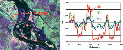Figure 13: The radiometric profile across the river from color composite of HH, HV and VV in RGB channel (Henry et al., 2006)

Comparisons and conclusions

In this paper the different methodology of flood extent mapping applied by different researchers both in active and passive remote sensing system together with their application examples have been presented. Comparing all these studies the following conclusions may be found:

• Flood mapping with Landsat TM or MSS is economic and might be applied for a large area. But due to lack of capability of TM or MSS sensor to penetrate through cloud and dense forest cover the method is weather dependent and unable to detect flood inundation beneath forest cover. The method applied by Wang et al (2002) used TM 4+TM 7 band to separate water from other land cover. They mentioned at TM 7 water might be distinguished from asphalt roads or rooftops but they didn’t provide any evidence in favor of this. However their method is efficient and economic.
• SAR data has the advantage of penetrate through cloud cover and forest canopies, but they require high cost. The difference image method of flood mapping using SAR data seems to more effective than the color composite method. The study of Lawrence et al. (2005) also implies that exists a good correlation between difference in flood inundation level and Radar backscatter values.
• Multi-polarized ASAR data may be used in more accurate flood mapping. HH polarizations provides a more suitable discrimination of flooded areas than HV and VV

References

• Henry, J.B., Chastanet, P., Fellah,K. and Desnos, Y.L., 2006, Envisat multi-polarized ASAR data for flood mapping, International Journal of Remote Sensing vol. 27, no. 10, 1921–1929
• Horritt, M. S., and Mason D. C., Flood boundary delineation from Synthetic Aperture Radar imagery using a statistical active contour model, International Journal of Remote Sensing, 2001, vol. 22, no. 13, 2489–2507
• Imhoff, M.L., Vermillon, C., Story, M.H., Choudhury, M.A., and Gafoor, A., 1987, Monsoon flood boundary delineation and damage assessment using space borne imaging radar and Landsat data, Photogrammetric Engineering and Remote Sensing, vol. 53 , 405-413
• Islam, M.M. and Sado, K., 2000a, Development of flood hazard maps of Bangladesh using NOAA-AVHRR images with GIS, Hydrological Sciences Journal, 45(3), 337-355
• Islam, M.M. and Sado, K., 2000b, Flood hazard assessment in Bangladesh using NOAA-AVHRR images with Geographic Information System, Hydrological Processes ,14, 605-620
• Islam, M.M. and Sado, K., 2002, Development of priority map for flood countermeasure by remote sensing data with Geographic Information System, Journal of Hydrologic Engineering, vol. 7, no. 5, 346-355
• Lawrence, M.K., Walker, N.D., Balasubramanian, S., Babin, A., and baras, J, 2005, Applications of Radarsat-1 synthetic aperture radar imagery to assess hurricane-related flooding of coastal Louisiana., International Journal of Remote Sensing, vol. 26, no. 24, 5359–5380
• Nghiem, S.V., Liu, W.T., Tsai, W.Y. and Xie, X., 2000, Flood mapping over the Asian continent during the 1999 summer monsoon season, Proceedings of IGARSS’00. IEEE Publication, pp. 2027-2028
• Townsend, P. A., ( 2002) , Relationships between forest structure and the detection of flood inundation in forested wetlands using C-band SAR, International Journal of Remote Sensing, vol. 23, no. 3, 443–460
• Wang, Y., Colby, J. D., and Mulcahy, K. A., 2002, An efficient method for mapping flood extent in a coastal floodplain using Landsat TM and DEM data, International Journal of Remote Sensing, vol. 23, no. 18, 3681–3696
• Wang, Y., 2004, Using Landsat 7 TM data acquired days after a flood event to delineate the maximum flood extent on a coastal floodplain, International Journal of Remote Sensing, vol. 25, no. 5, 959–974

NB: This article entitled 'Determination of Flood Extent Using Remote Sensing' has been submitted as a term paper at University of Alberta by the author (Zahidul Islam), Ph.D. Candidate, Department of Civil and Environmental Engineering, University of Alberta in 2007. Copying any part of this article is completely prohibitive and would be considered as the violation of copyright.